
Cross validation
Rafael Irizarry
A common goal of machine learning is to find an algorithm that produces predictors for an outcome that minimizes the MSE:

When all we have at our disposal is one dataset, we can estimate the MSE with the observed MSE like this:

These two are often referred to as the true error and apparent error, respectively.
There are two important characteristics of the apparent error we should always keep in mind:
- Because our data is random, the apparent error is a random variable. For example, the dataset we have may be a random sample from a larger population. An algorithm may have a lower apparent error than another algorithm due to luck.
- If we train an algorithm on the same dataset that we use to compute the apparent error, we might be overtraining. In general, when we do this, the apparent error will be an underestimate of the true error. We will see an extreme example of this with k-nearest neighbors.
Cross validation is a technique that permits us to alleviate both these problems. To understand cross validation, it helps to think of the true error, a theoretical quantity, as the average of many apparent errors obtained by applying the algorithm to  new random samples of the data, none of them used to train the algorithm. As shown in a previous chapter, we think of the true error as:

with a large number that can be thought of as practically infinite. As already mentioned, this is a theoretical quantity because we only have available one set of outcomes:  . Cross validation is based on the idea of imitating the theoretical setup above as best we can with the data we have. To do this, we have to generate a series of different random samples. There are several approaches we can use, but the general idea for all of them is to randomly generate smaller datasets that are not used for training, and instead used to estimate the true error.
K-fold cross validation
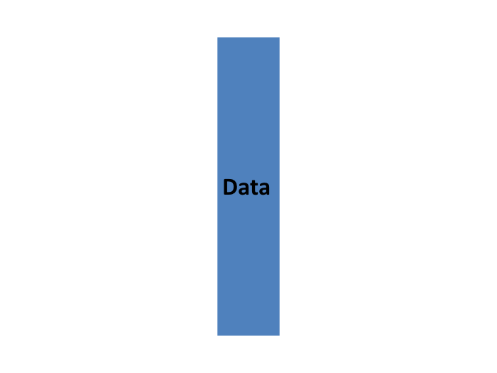
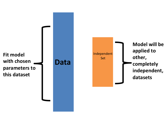
The first one we describe is K-fold cross validation. Generally speaking, a machine learning challenge starts with a dataset (blue in the image below). We need to build an algorithm using this dataset that will eventually be used in completely independent datasets (yellow).
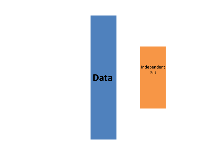
But we don’t get to see these independent datasets.
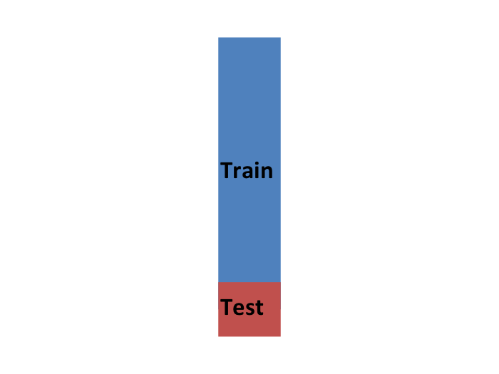
So to imitate this situation, we carve out a piece of our dataset and pretend it is an independent dataset: we divide the dataset into a training set (blue) and a test set (red). We will train our algorithm exclusively on the training set and use the test set only for evaluation purposes.
We usually try to select a small piece of the dataset so that we have as much data as possible to train. However, we also want the test set to be large so that we obtain a stable estimate of the loss without fitting an impractical number of models. Typical choices are to use 10%-20% of the data for testing.
Let’s reiterate that it is indispensable that we not use the test set at all: not for filtering out rows, not for selecting features, nothing!
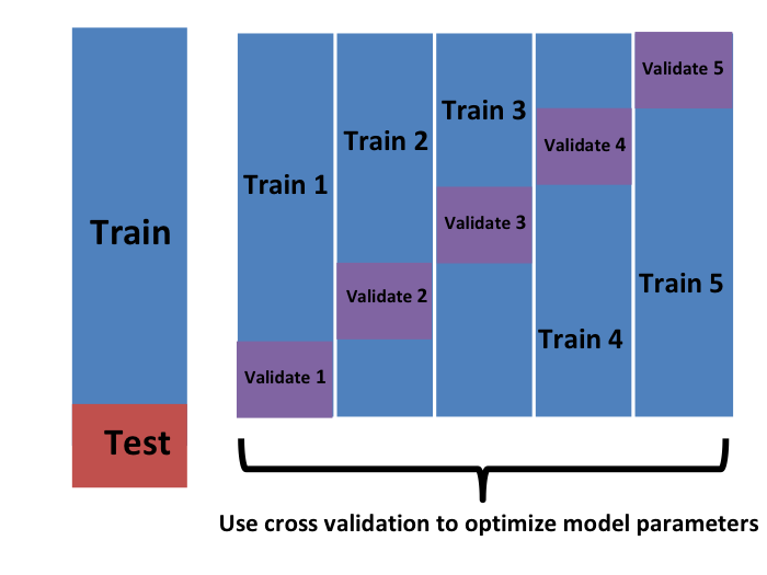
Now this presents a new problem because for most machine learning algorithms we need to select parameters, for example the number of neighbors  in k-nearest neighbors. Here, we will refer to the set of parameters as
  . We need to optimize algorithm parameters without using our test set and we know that if we optimize and evaluate on the same dataset, we will overtrain. This is where cross validation is most useful.
For each set of algorithm parameters being considered, we want an estimate of the MSE and then we will choose the parameters with the smallest MSE. Cross validation provides this estimate.
First, before we start the cross validation procedure, it is important to fix all the algorithm parameters. Although we will train the algorithm on the set of training sets, the parameters will be the same across all training sets. We will use  to denote the predictors obtained when we use parameters .
So, if we are going to imitate this definition:

we want to consider datasets that can be thought of as an independent random sample and we want to do this several times. With K-fold cross validation, we do it  times. In the cartoons, we are showing an example that uses
  .
.
We will eventually end up with samples, but let’s start by describing how to construct the first: we simply pick  observations at random (we round if
  is not a round number) and think of these as a random sample
  with
with  . We call this the validation set:
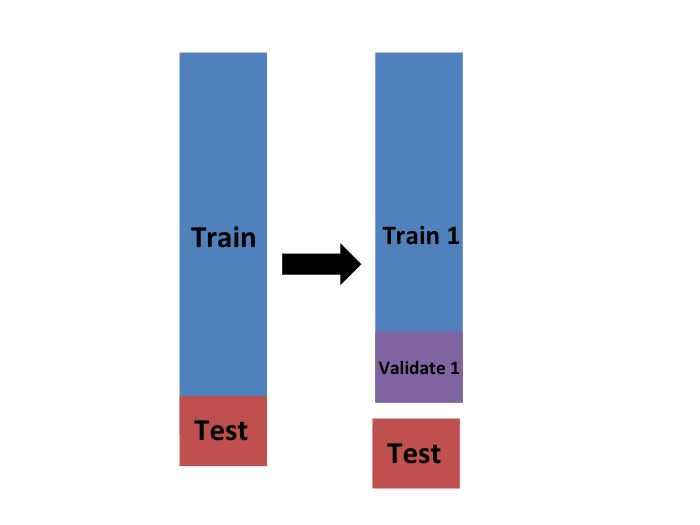
Now we can fit the model in the training set, then compute the apparent error on the independent set:

Note that this is just one sample and will therefore return a noisy estimate of the true error. This is why we take samples, not just one. In K-cross validation, we randomly split the observations into non-overlapping sets:
Now we repeat the calculation above for each of these sets  and obtain
  . Then, for our final estimate, we compute the average:

and obtain an estimate of our loss. A final step would be to select the that minimizes the MSE.
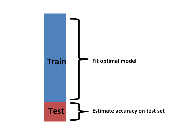
We have described how to use cross validation to optimize parameters. However, we now have to take into account the fact that the optimization occurred on the training data and therefore we need an estimate of our final algorithm based on data that was not used to optimize the choice. Here is where we use the test set we separated early on:
We can do cross validation again:
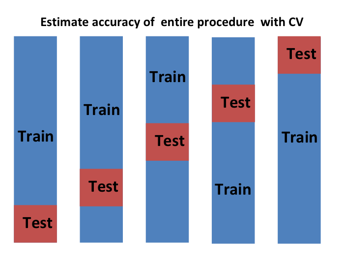
and obtain a final estimate of our expected loss. However, note that this means that our entire compute time gets multiplied by . You will soon learn that performing this task takes time because we are performing many complex computations. As a result, we are always looking for ways to reduce this time. For the final evaluation, we often just use the one test set.
Once we are satisfied with this model and want to make it available to others, we could refit the model on the entire dataset, without changing the optimized parameters.
Now how do we pick the cross validation ? Large values of are preferable because the training data better imitates the original dataset. However, larger values of will have much slower computation time: for example, 100-fold cross validation will be 10 times slower than 10-fold cross validation. For this reason, the choices of and  are popular.
One way we can improve the variance of our final estimate is to take more samples. To do this, we would no longer require the training set to be partitioned into non-overlapping sets. Instead, we would just pick sets of some size at random.
One popular version of this technique, at each fold, picks observations at random with replacement (which means the same observation can appear twice). This approach has some advantages (not discussed here) and is generally referred to as the bootstrap. In fact, this is the default approach in the caret package. We describe how to implement cross validation with the caret package in the next chapter. In the next section, we include an explanation of how the bootstrap works in general.
