
Feature Visualization
Christoph Molnar
The approach of making the learned features explicit is called Feature Visualization. Feature visualization for a unit of a neural network is done by finding the input that maximizes the activation of that unit.
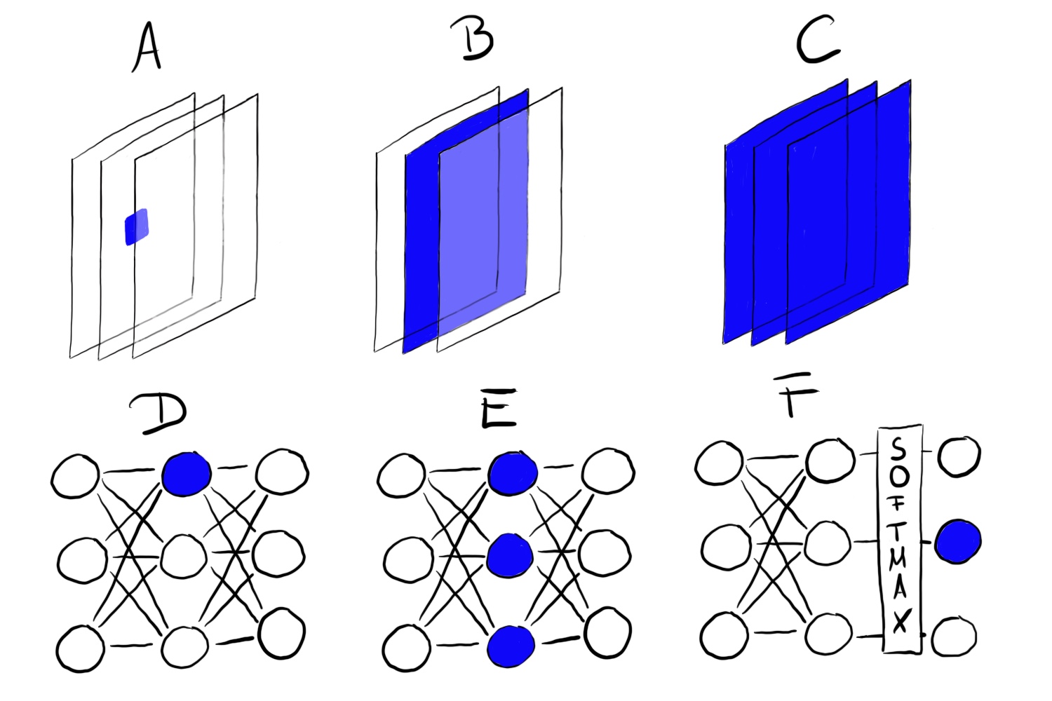
“Unit” refers either to individual neurons, channels (also called feature maps), entire layers or the final class probability in classification (or the corresponding pre-softmax neuron, which is recommended). Individual neurons are atomic units of the network, so we would get the most information by creating feature visualizations for each neuron. But there is a problem: Neural networks often contain millions of neurons. Looking at each neuron’s feature visualization would take too long. The channels (sometimes called activation maps) as units are a good choice for feature visualization. We can go one step further and visualize an entire convolutional layer. Layers as a unit are used for Google’s DeepDream, which repeatedly adds the visualized features of a layer to the original image, resulting in a dream-like version of the input.
Feature Visualization through Optimization
In mathematical terms, feature visualization is an optimization problem. We assume that the weights of the neural network are fixed, which means that the network is trained. We are looking for a new image that maximizes the (mean) activation of a unit, here a single neuron:

The function ℎ is the activation of a neuron, img the input of the network (an image), x and y describe the spatial position of the neuron, n specifies the layer and z is the channel index. For the mean activation of an entire channel z in layer n we maximize:

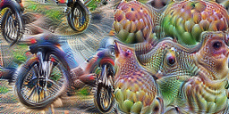
In this formula, all neurons in channel z are equally weighted. Alternatively, you can also maximize random directions, which means that the neurons would be multiplied by different parameters, including negative directions. In this way, we study how the neurons interact within the channel. Instead of maximizing the activation, you can also minimize it (which corresponds to maximizing the negative direction). Interestingly, when you maximize the negative direction you get very different features for the same unit:
We can address this optimization problem in different ways. For example, instead of generating new images, we could search through our training images and select those that maximize the activation. This is a valid approach, but using training data has the problem that elements on the images can be correlated and we cannot see what the neural network is really looking for. If images that yield a high activation of a certain channel show a dog and a tennis ball, we do not know whether the neural network looks at the dog, the tennis ball or maybe at both.
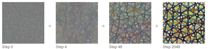
Another approach is to generate new images, starting from random noise. To obtain meaningful visualizations, there are usually constraints on the image, e.g. that only small changes are allowed. To reduce noise in the feature visualization, you can apply jittering, rotation or scaling to the image before the optimization step. Other regularization options include frequency penalization (e.g. reduce variance of neighboring pixels) or generating images with learned priors, e.g. with generative adversarial networks (GANs) [1] or denoising autoencoders [2].
If you want to dive a lot deeper into feature visualization, take a look at the distill.pub online journal, especially the feature visualization post by Olah et al. (2017) [3], from which I used many of the images. I also recommend the article about the building blocks of interpretability [4].
Connection to Adversarial Examples
There is a connection between feature visualization and adversarial examples: Both techniques maximize the activation of a neural network unit. For adversarial examples, we look for the maximum activation of the neuron for the adversarial (= incorrect) class. One difference is the image we start with: For adversarial examples, it is the image for which we want to generate the adversarial image. For feature visualization it is, depending on the approach, random noise.
Text and Tabular Data
The literature focuses on feature visualization for convolutional neural networks for image recognition. Technically, there is nothing to stop you from finding the input that maximally activates a neuron of a fully connected neural network for tabular data or a recurrent neural network for text data. You might not call it feature visualization any longer, since the “feature” would be a tabular data input or text. For credit default prediction, the inputs might be the number of prior credits, number of mobile contracts, address and dozens of other features. The learned feature of a neuron would then be a certain combination of the dozens of features. For recurrent neural networks, it is a bit nicer to visualize what the network learned: Karpathy et al. (2015)[5]showed that recurrent neural networks indeed have neurons that learn interpretable features. They trained a character-level model, which predicts the next character in the sequence from the previous characters. Once an opening brace “(” occurred, one of the neurons got highly activated, and got de-activated when the matching closing bracket “)” occurred. Other neurons fired at the end of a line. Some neurons fired in URLs. The difference to the feature visualization for CNNs is that the examples were not found through optimization, but by studying neuron activations in the training data.
- Nguyen, Anh, Alexey Dosovitskiy, Jason Yosinski, Thomas Brox, and Jeff Clune. “Synthesizing the preferred inputs for neurons in neural networks via deep generator networks.” Advances in neural information processing systems 29 (2016): 3387-3395. ↵
- Nguyen, Anh, Jeff Clune, Yoshua Bengio, Alexey Dosovitskiy, and Jason Yosinski. “Plug & play generative networks: Conditional iterative generation of images in latent space.” In Proceedings of the IEEE Conference on Computer Vision and Pattern Recognition, pp. 4467-4477. 2017. ↵
- Olah, Chris, Alexander Mordvintsev, and Ludwig Schubert. “Feature visualization.” Distill 2, no. 11 (2017): e7. ↵
- Olah, Chris, Arvind Satyanarayan, Ian Johnson, Shan Carter, Ludwig Schubert, Katherine Ye, and Alexander Mordvintsev. “The building blocks of interpretability.” Distill 3, no. 3 (2018): e10. ↵
- Karpathy, Andrej, Justin Johnson, and Li Fei-Fei. “Visualizing and understanding recurrent networks.” arXiv preprint arXiv:1506.02078 (2015). ↵
