
Plots for two variables
Rafael Irizarry
In general, you should use scatterplots to visualize the relationship between two variables. In every single instance in which we have examined the relationship between two variables, including total murders versus population size, life expectancy versus fertility rates, and infant mortality versus income, we have used scatterplots. This is the plot we generally recommend. However, there are some exceptions and we describe two alternative plots here: the slope chart and the Bland-Altman plot.
Slope charts
One exception where another type of plot may be more informative is when you are comparing variables of the same type, but at different time points and for a relatively small number of comparisons. For example, comparing life expectancy between 2010 and 2015. In this case, we might recommend a slope chart. Below is an example comparing 2010 to 2015 for large western countries:
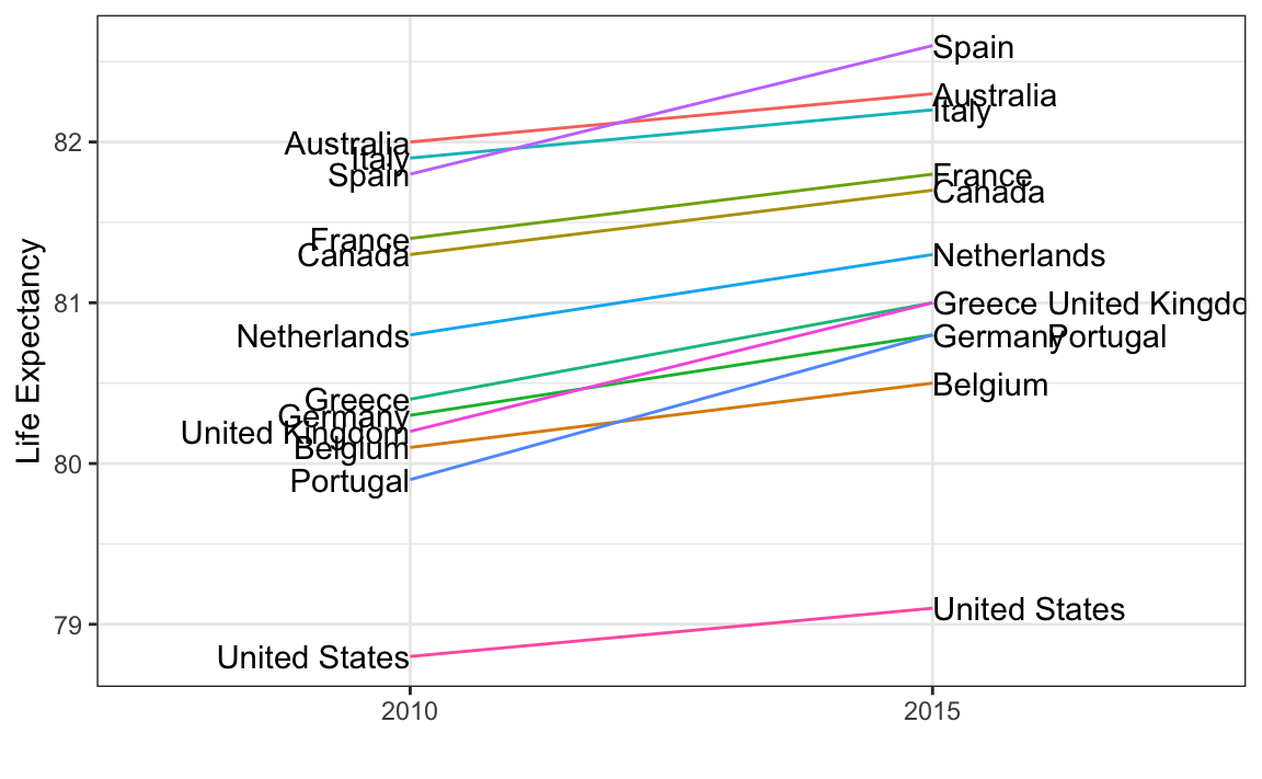
An advantage of the slope chart is that it permits us to quickly get an idea of changes based on the slope of the lines. Although we are using angle as the visual cue, we also have position to determine the exact values. Comparing the improvements is a bit harder with a scatterplot:
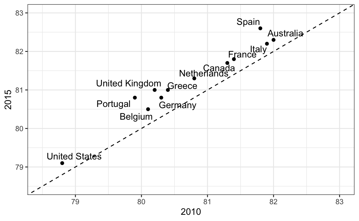
In the scatterplot, we have followed the principle use common axes since we are comparing these before and after. However, if we have many points, slope charts stop being useful as it becomes hard to see all the lines.
Bland-Altman plot
Since we are primarily interested in the difference, it makes sense to dedicate one of our axes to it. The Bland-Altman plot, also known as the Tukey mean-difference plot and the MA-plot, shows the difference versus the average:
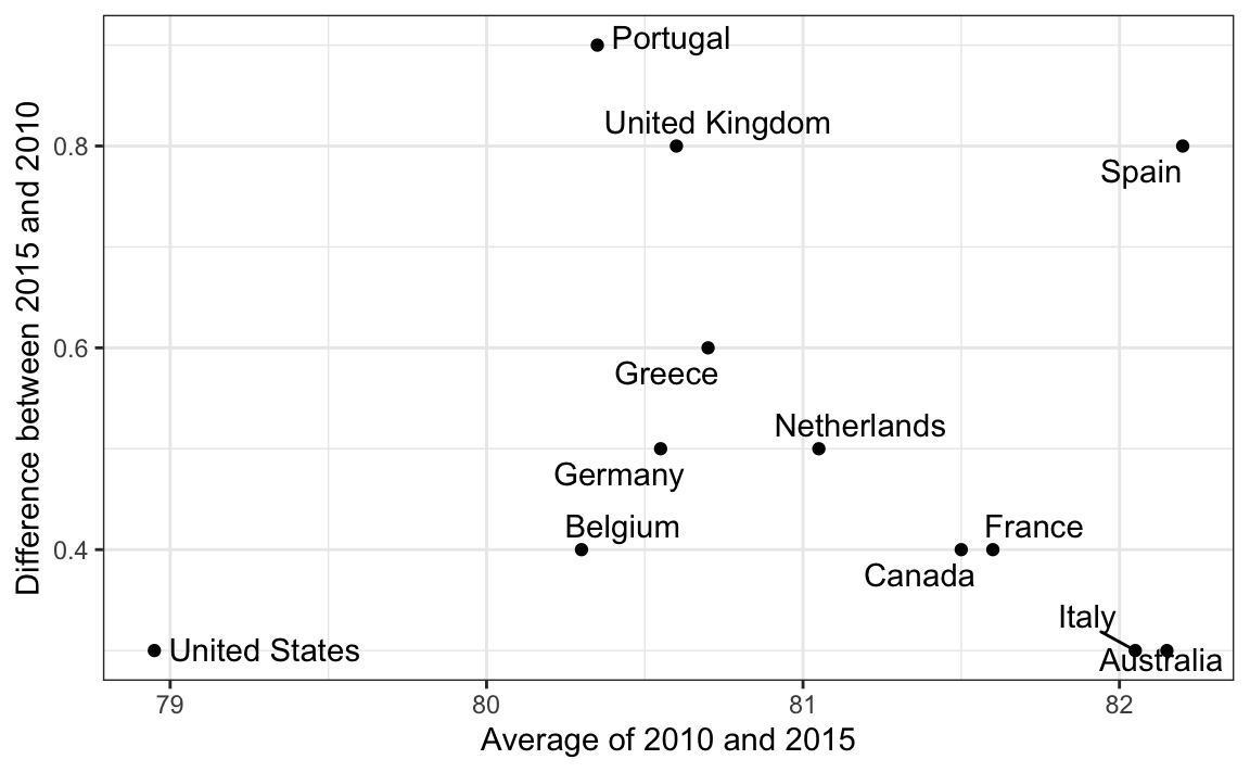
Here, by simply looking at the y-axis, we quickly see which countries have shown the most improvement. We also get an idea of the overall value from the x-axis.
