Random forests

Random forests are a very popular machine learning approach that addresses the shortcomings of decision trees using a clever idea. The goal is to improve prediction performance and reduce instability by averaging multiple decision trees (a forest of trees constructed with randomness). It has two features that help accomplish this.

The first step is bootstrap aggregation or bagging. The general idea is to generate many predictors, each using regression or classification trees, and then forming a final prediction based on the average prediction of all these trees. To assure that the individual trees are not the same, we use the bootstrap to induce randomness. These two features combined explain the name: the bootstrap makes the individual trees randomly different, and the combination of trees is the forest. The specific steps are as follows.

1. Build decision trees using the training set. We refer to the fitted models as . We later explain how we ensure they are different.

2. For every observation in the test set, form a prediction using tree .

3. For continuous outcomes, form a final prediction with the average . For categorical data classification, predict  with majority vote (most frequent class among ).

So how do we get different decision trees from a single training set? For this, we use randomness in two ways which we explain in the steps below. Let be the number of observations in the training set. To create  from the training set we do the following:

1. Create a bootstrap training set by sampling  observations from the training set with replacement. This is the first way to induce randomness.

2. A large number of features is typical in machine learning challenges. Often, many features can be informative but including them all in the model may result in overfitting. The second way random forests induce randomness is by randomly selecting features to be included in the building of each tree. A different random subset is selected for each tree. This reduces correlation between trees in the forest, thereby improving prediction accuracy.

To illustrate how the first steps can result in smoother estimates we will demonstrate by fitting a random forest to the 2008 polls data.

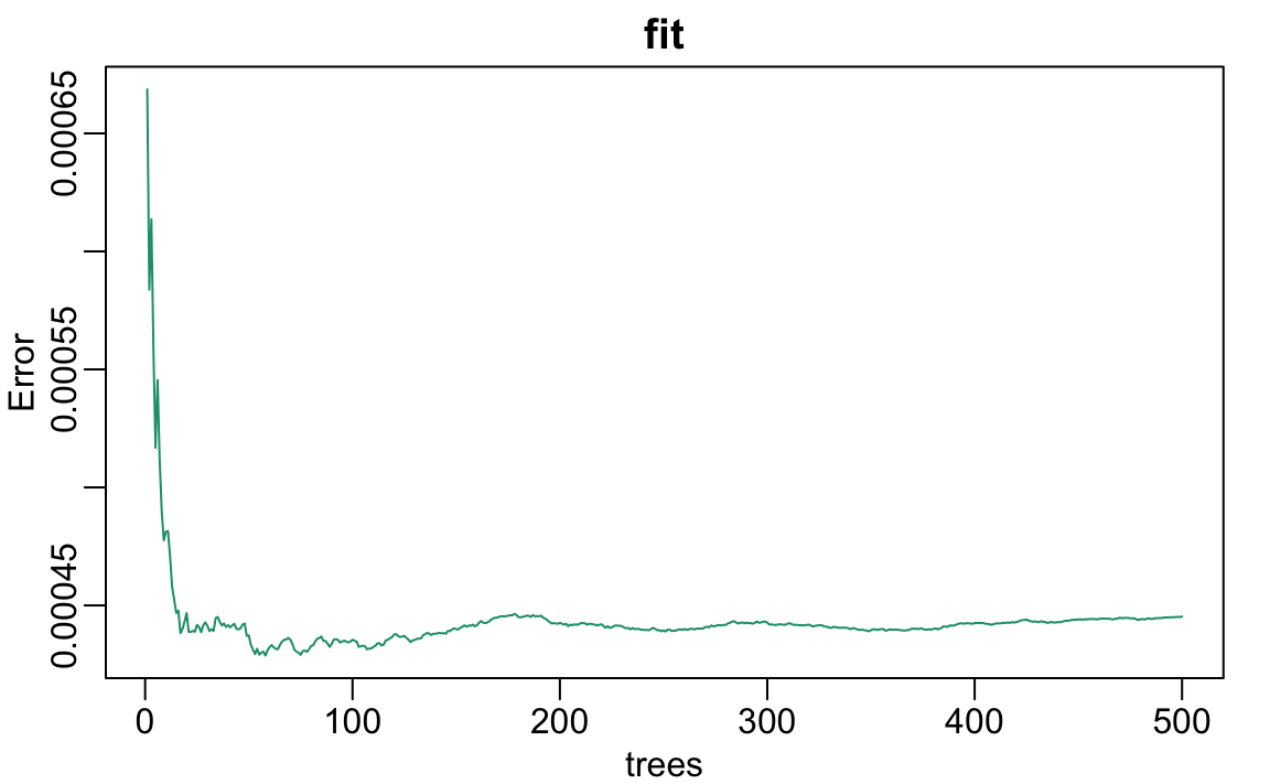
We can see that in this case, the accuracy improves as we add more trees until about 30 trees where accuracy stabilizes.

The resulting estimate for this random forest can be seen like this.

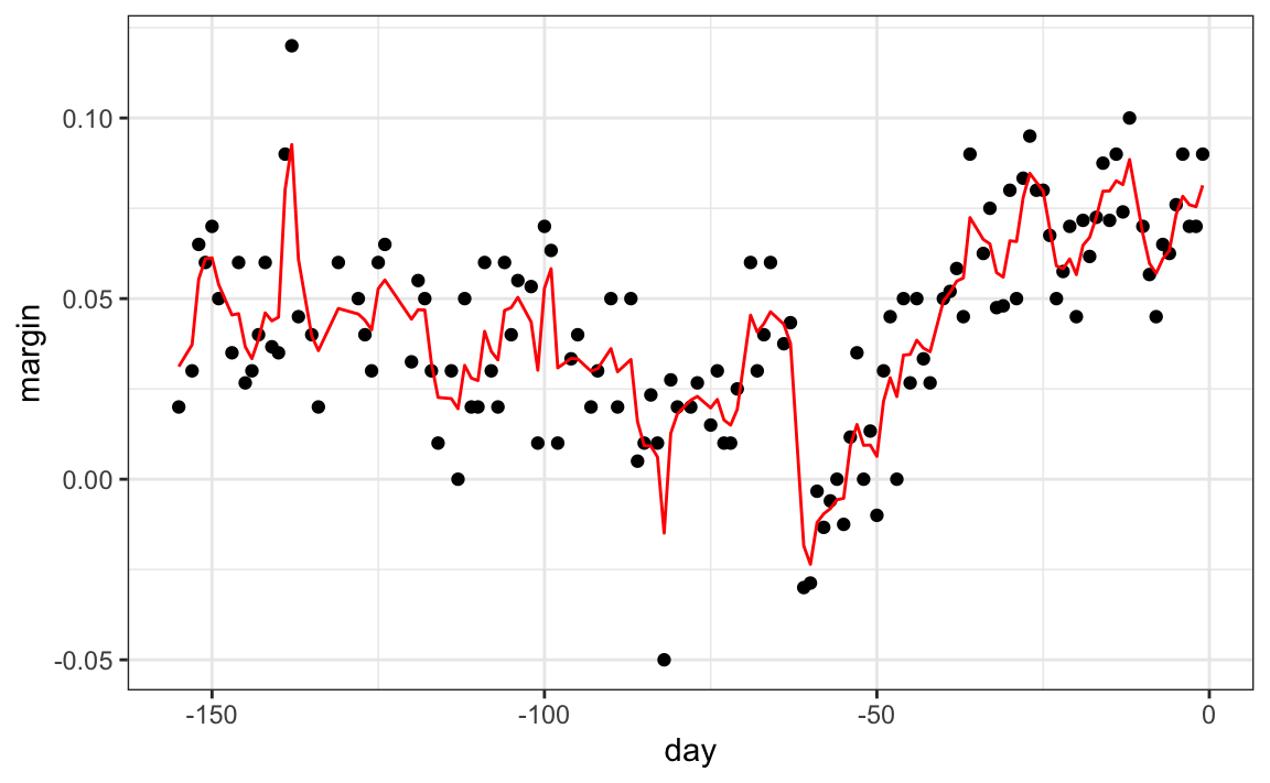
Notice that the random forest estimate is much smoother than what we achieved with the regression tree in the previous section. This is possible because the average of many step functions can be smooth. We can see this by visually examining how the estimate changes as we add more trees. In the following figure you see each of the bootstrap samples for several values of  and for each one we see the tree that is fitted in grey, the previous trees that were fitted in lighter grey, and the result of averaging all the trees estimated up to that point.

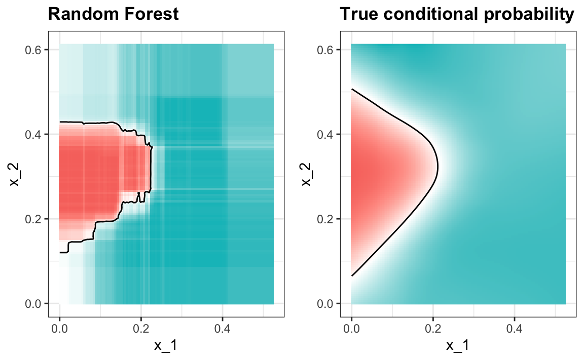
Here is what the conditional probabilities look like.

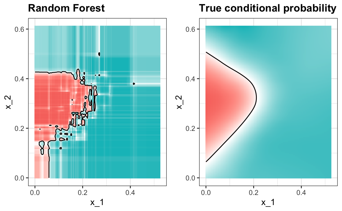
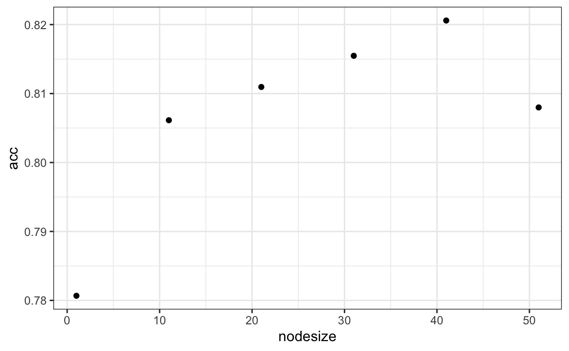
Visualizing the estimate shows that, although we obtain high accuracy, it appears that there is room for improvement by making the estimate smoother. This could be achieved by changing the parameter that controls the minimum number of data points in the nodes of the tree. The larger this minimum, the smoother the final estimate will be. We can train the parameters of the random forest. Below, we can optimize over the minimum node size.

We can now fit the random forest with the optimized minimum node size to the entire training data and evaluate performance on the test data. The selected model improves accuracy and provides a smoother estimate.

Random forest performs better in all the examples we have considered. However, a disadvantage of random forests is that we lose interpretability. An approach that helps with interpretability is to examine variable importance. To define variable importance we count how often a predictor is used in the individual trees. You can learn more about variable importance in an advanced machine learning book^[1].