Sensitivity and specificity

Rafael Irizarry

Sensitivity and specificity

Rafael Irizarry

To define sensitivity and specificity, we need a binary outcome. When the outcomes are categorical, we can define these terms for a specific category. In the digits example, we can ask for the specificity in the case of correctly predicting 2 as opposed to some other digit. Once we specify a category of interest, then we can talk about positive outcomes, $Y=1$ , and negative outcomes $Y=0$ .

In general, sensitivity is defined as the ability of an algorithm to predict a positive outcome when the actual outcome is positive: $\hat{Y}=1$ when $Y=1$ . Because an algorithm that calls everything positive ( $\hat{Y}=1$ no matter what) has perfect sensitivity, this metric on its own is not enough to judge an algorithm. For this reason, we also examine specificity, which is generally defined as the ability of an algorithm to not predict a positive $\hat{Y}=0$ when the actual outcome is not a positive $Y=0$ . We can summarize in the following way:

High sensitivity: $Y = 1\Longrightarrow\hat{Y}=1$
High specificity: $Y = 0\Longrightarrow\hat{Y}=0$

Although the above is often considered the definition of specificity, another way to think of specificity is by the proportion of positive calls that are actually positive:

High specificity: $\hat{Y} = 1\LongrightarrowY=1$ .

To provide precise definitions, we name the four entries of the confusion matrix:

	Actually Positive	Actually Negative
Predicted positive	True positives (TP)	False positives (FP)
Predicted negative	False negatives (FN)	True negatives (TN)

Sensitivity is typically quantified by $TP/(TP+FN)$ , the proportion of actual positives (the first column = $TP+FN$ ) that are called positives ( $TP$ ). This quantity is referred to as the true positive rate (TPR) or recall.

Specificity is defined as $TN/(TN+FP)$ or the proportion of negatives (the second column = $FP+TN$ ) that are called negatives ( $TN$ ). This quantity is also called the true negative rate (TNR). There is another way of quantifying specificity which is $TP/(TP+FP)$ or the proportion of outcomes called positives (the first row or $TP+FP$ ) that are actually positives ( $TP$ . This quantity is referred to as positive predictive value (PPV) and also as precision. Note that, unlike TPR and TNR, precision depends on prevalence since higher prevalence implies you can get higher precision even when guessing.

The multiple names can be confusing, so we include a table to help us remember the terms. The table includes a column that shows the definition if we think of the proportions as probabilities.

Measure of	Name 1	Name 2	Definition	Probability representation
sensitivity	TPR	Recall	$\frac{TP}{TP + FN}$	$Pr (\hat{Y} = 1 ∣ Y = 1)$
specificity	TNR	1-FPR	$\frac{TN}{TN + FP}$	$Pr (\hat{Y} = 0 ∣ Y = 0)$
specificity	PPV	Precision	$\frac{TP}{TP + FP}$	$Pr (Y = 1 ∣ \hat{Y} = 1)$

Here TPR is True Positive Rate, FPR is False Positive Rate, and PPV is Positive Predictive Value. The caret function confusionMatrix computes all these metrics for us once we define what category “positive” is. The function expects factors as input, and the first level is considered the positive outcome or $Y=1$ . In our example, Female is the first level because it comes before Male alphabetically. If you type this into R you will see several metrics including accuracy, sensitivity, specificity, and PPV.

We can see that the high overall accuracy is possible despite relatively low sensitivity. As we hinted at above, the reason this happens is because of the low prevalence (0.23): the proportion of females is low. Because prevalence is low, failing to predict actual females as females (low sensitivity) does not lower the accuracy as much as failing to predict actual males as males (low specificity). This is an example of why it is important to examine sensitivity and specificity and not just accuracy. Before applying this algorithm to general datasets, we need to ask ourselves if prevalence will be the same.

Balanced accuracy and F1 score

Although we usually recommend studying both specificity and sensitivity, very often it is useful to have a one-number summary, for example for optimization purposes. One metric that is preferred over overall accuracy is the average of specificity and sensitivity, referred to as balanced accuracy. Because specificity and sensitivity are rates, it is more appropriate to compute the harmonic average. In fact, the $F_{1}$ -score, a widely used one-number summary, is the harmonic average of precision and recall:

$\frac{1}{\frac{1}{2}\left(\frac{1}{\mbox{recall}} + \frac{1}{\mbox{precision}}\right) }$

Because it is easier to write, you often see this harmonic average rewritten as:

$2 \times \frac{\mbox{precision} \cdot \mbox{recall}} {\mbox{precision} + \mbox{recall}}$

when defining $F_{1}$ .

Remember that, depending on the context, some types of errors are more costly than others. For example, in the case of plane safety, it is much more important to maximize sensitivity over specificity: failing to predict a plane will malfunction before it crashes is a much more costly error than grounding a plane when, in fact, the plane is in perfect condition. In a capital murder criminal case, the opposite is true since a false positive can lead to executing an innocent person. The $F_1$ -score can be adapted to weigh specificity and sensitivity differently. To do this, we define $\beta$ to represent how much more important sensitivity is compared to specificity and consider a weighted harmonic average:

$\frac{1}{\frac{\beta^2}{1+\beta^2}\frac{1}{\mbox{recall}} + \frac{1}{1+\beta^2}\frac{1}{\mbox{precision}} }$

Let’s rebuild our prediction algorithm, but this time maximizing the F-score instead of overall accuracy:

As before, we can plot these $F_1$ measures versus the cutoffs:

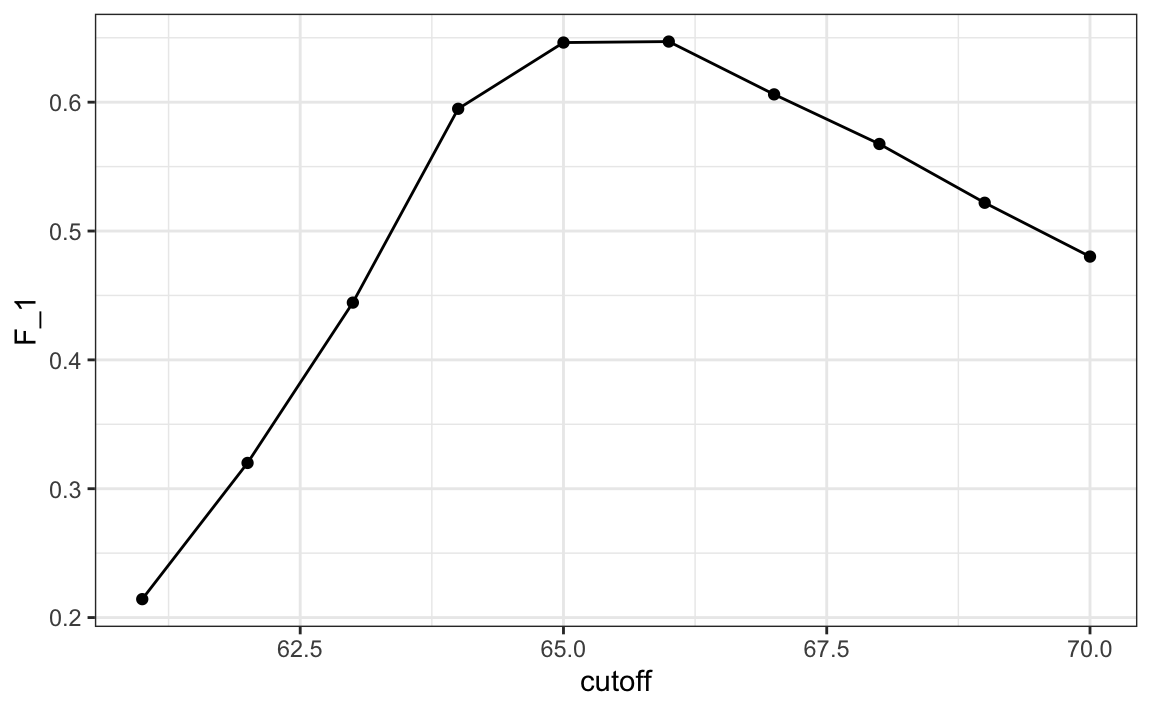
A line dot graph showing context between F1 measures and cutoffs. The graph increases slowly before plateauing and declining quickly. — The relationship between F1 measures and cutoff.

A cutoff of 66 makes more sense than 64. Furthermore, it balances the specificity and sensitivity of our confusion matrix.

License

Icon for the Creative Commons Attribution-NonCommercial-ShareAlike 4.0 International License

Balanced accuracy and F1 score

License

Share This Book